“AI” How to Construct LSTM Model with Multiple Input & Output Dimension.

 

In this page, I introduce how to construct LSTM model that has multiple input and output dimension by using tensorflow-keras.

 

OK, let’s get started!!

 

Prepare Sample Data for AI Model

At first, let’s prepare sample data to construct LSTM model.

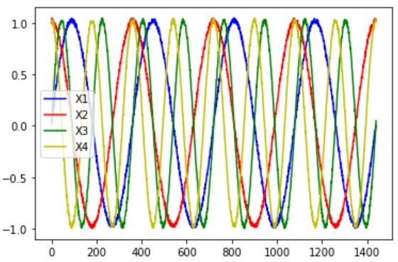
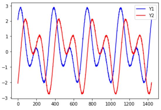
This time, I use easy SIN & COS wave data for input (total 4 data) and composite wave of these for output (total 2 data) .

 

Below is the sample code of construct base wave data.

import numpy as np
xdeg=1440
x = np.arange(0,xdeg+1)
sinx=np.sin(2*np.pi*x/360)+np.random.rand(len(x))/20
sin2x=np.sin(2*2*np.pi*x/360)+np.random.rand(len(x))/20
cosx=np.cos(2*np.pi*x/360)+np.random.rand(len(x))/20
cos2x=np.cos(2*2*np.pi*x/360)+np.random.rand(len(x))/20

These wave data has total 0~1440 degree and it is per 1 degree.

 

Let’s confirm inside of “sinx”.

It is 1 dimension data like this.

 

The prerequisite of sample code shown after is all data is one dimension.

 

Anyway, let’s construct input and output data for LSTM model.

X1=sinx
X2=cosx
X3=sin2x
X4=cos2x
Y1=X1+X2+X3+X4
Y2=X1-X2+X3-X4

X1~X4 is used as input and Y1,Y2 is used as output in LSTM model.

 

Let’s make figure of these data.

import matplotlib.pyplot as plt
plt.plot(range(0, len(x)), X1, color="b", label="X1")
plt.plot(range(0, len(x)), X2, color="r", label="X2")
plt.plot(range(0, len(x)), X3, color="g", label="X3")
plt.plot(range(0, len(x)), X4, color="y", label="4")
plt.legend()
plt.show()
plt.plot(range(0, len(x)), Y1, color="b", label="Y1")
plt.plot(range(0, len(x)), Y2, color="r", label="Y2")
plt.legend()
plt.show()

★Input Data (X1~X4))

★Output Data (Y1,Y2)

Pre-Process Data for LSTM model

Next, let’s conduct pre-process data for LSTM model.

 

Input data is time series data of X1~X4 and output data is next one time data of Y1,Y2.

This time, number of time series data is 5 (set in “look_back”) .

X_list=[X1,X2,X3,X4]
Y_list=[Y1,Y2]
Xdata=[]
Ydata=[]
look_back=5
for i in range(len(x)-look_back):
    Xtimedata=[]
    for j in range(len(X_list)):
        Xtimedata.append(X_list[j][i:i+look_back])
    Xtimedata=np.array(Xtimedata)
    Xtimedata=Xtimedata.transpose()
    Xdata.append(Xtimedata)
    Ytimedata=[]
    for j in range(len(Y_list)):
        Ytimedata.append(Y_list[j][i+look_back])
    Ydata.append(Ytimedata)
Xdata=np.array(Xdata)
Ydata=np.array(Ydata)

By conduct this program, input data is stored in “Xdata” and output data is stored in “Ydata” and LSTM model can receive as it is.

 

Construct LSTM Model has Multiple In-Out Dimension

OK, let’s construct LSTM model by using prepared data above.

 

The sample code is below.

from tensorflow.keras.models import Sequential
from tensorflow.keras.layers import Dense, Activation
from tensorflow.keras.layers import LSTM
from tensorflow.keras.optimizers import Adam
Xdim=Xdata.shape[2]
Ydim=Ydata.shape[1]
validation_split_rate=0.2
model = Sequential()
model.add(LSTM(4, input_shape=(look_back,Xdim)))
model.add(Dense(Ydim))
model.compile(loss="mean_squared_error", optimizer=Adam(lr=0.001))
model.summary()
history=model.fit(Xdata,Ydata,batch_size=16,epochs=100,validation_split=validation_split_rate)

Learning started like this.

 

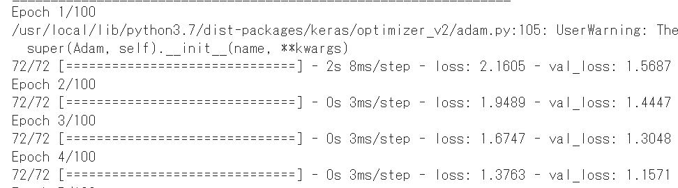
I think you can understand how to construct LSTM model has multiple input and output dimension.

 

Confirm Model Loss and Prediction Accuracy

On the occasion, let’s confirm model loss and prediction accuracy.

At first, below is the code for plot of model loss.

plt.plot(history.history['loss'])
plt.plot(history.history['val_loss'])
plt.title('Model loss')
plt.ylabel('Loss')
plt.xlabel('Epoch')
plt.legend(['Train', 'Test'], loc='upper left')
plt.show()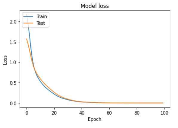

I think you can confirm loss decrease without a problem.

 

Next is confirm prediction accuracy.

The data that is not used as learning data is used for prediction accuracy.

Xdata_validation=Xdata[-int(len(Xdata)*(validation_split_rate)):]
Ydata_validation=Ydata[-int(len(Ydata)*(validation_split_rate)):]
Predictdata = model.predict(Xdata_validation)
plt.plot(range(0, len(Predictdata)),Predictdata[:,0], color="b", label="predict")
plt.plot(range(0, len(Ydata_validation)),Ydata_validation[:,0], color="r", label="row_data")
plt.legend()
plt.show()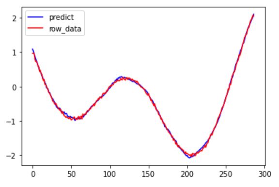

This is also no problem.

 

That’s all. Thank you!!