Hi, this is Higashi.
When you create a chart in Python, Plotly lets you zoom in with the mouse and hover over a line to read its values.
But tutorials often mention saving the chart as HTML or displaying it in a browser. If we’re making a chart with Python, why do we need HTML and a browser?
This time I’ll go through how a Plotly chart gets displayed, then show what you can do with one.
- Python and JavaScript share the work
- What do HTML, JavaScript, and the browser do?
- What’s inside a Python Figure?
- Passing the data and settings to Plotly.js
- Saving as HTML lets you interact after Python closes
- In Jupyter, the output cell is the display area
- Does Python run again every time you zoom?
- Trying it with a sine wave
- Here’s what you can do with it
Python and JavaScript share the work
We’re using the Python Plotly library. Python code lets you specify the data, line colors, axis labels, and other chart settings.
Drawing the chart on screen and responding to the mouse are handled by Plotly.js, a JavaScript library.
The process looks like this.
Python
Prepare the data and chart settings
                ↓
Pass the data and settings to the display environment
                ↓
Plotly.js
Draw the chart and respond to mouse interactions
The results calculated in Python are passed to Plotly.js, which turns them into a chart you can interact with in a browser or a similar display environment.
What do HTML, JavaScript, and the browser do?
Here’s what each part does in this example.
| Part | Role in the chart |
|---|---|
| HTML | Provides the page structure and a place to display the chart. |
| JavaScript | Draws the chart and responds to mouse interactions. |
| Browser | Reads the HTML and runs the JavaScript to display the result. |
For example, when values appear as you hover over a chart, JavaScript handles that interaction.
Plotly.js provides the code for these features. Using Plotly from Python lets you create an interactive chart without writing the JavaScript mouse handlers yourself.
What’s inside a Python Figure?
You’ll often see these lines in Plotly examples.
import plotly.graph_objects as go

figure = go.Figure()
A Figure is an object that holds the chart’s data and settings.
| Information | What it specifies |
|---|---|
| Data traces | The x and y values, chart type such as a line or scatter plot, and trace names. |
| Layout | The chart title, axis labels, legend position, and visible ranges. |
For example, this code adds three data points.
figure.add_trace(
    go.Scatter(
        x=[0, 1, 2],
        y=[0, 1, 0],
        mode="lines",
        name="Sample",
    )
)
add_trace adds a data series to the chart. Here, the x values are 0, 1, and 2, and the y values are 0, 1, and 0, connected by lines. At this point, Python has the information describing what the chart should show.
Passing the data and settings to Plotly.js
To display the chart, the data and settings in the Python Figure are converted into a form that JavaScript can use.
This uses JSON, a format that represents data through names and values. A simplified version of the previous example looks like this.
{
  "data": [
    {
      "type": "scatter",
      "x": [0, 1, 2],
      "y": [0, 1, 0],
      "mode": "lines",
      "name": "Sample"
    }
  ]
}
Plotly.js reads this information and draws the lines at the specified coordinates. The values prepared in Python also reach the display environment as data, so the chart can show them when you hover over it. Plotly documentation on figure structure
Saving as HTML lets you interact after Python closes
You can save the chart as an HTML file with this code.
figure.write_html(
    "interactive_graph.html",
    include_plotlyjs=True,
)
This setting includes the chart’s data, settings, and Plotly.js in the HTML file.
Opening that file in a browser displays the chart using the data and JavaScript inside it. For a chart like this one, you can still zoom, pan, and inspect values after closing Python.
Since the file includes the JavaScript it needs, this example also works offline. Including that JavaScript makes the HTML file larger. Plotly documentation on HTML export
In Jupyter, the output cell is the display area
In Jupyter Notebook or JupyterLab, you can display the chart like this.
figure.show()The chart appears in the cell’s output area. Plotly.js still draws the chart and handles mouse interactions in that display area.
Where figure.show() displays a chart depends on your Python environment and renderer settings. A regular Python script can also be configured to open the chart in a browser. Plotly documentation on renderers
Does Python run again every time you zoom?
For a chart like this, with the data already passed to the display environment, zooming doesn’t require Python to run again.
Plotly.js handles displaying the area you select by dragging and showing the values of points near the mouse.
If you want to change an input, rerun a Python simulation, and update the chart with its results, you’ll need to connect the interface to that Python calculation. Dash, which builds web apps with Plotly, and widgets in Jupyter are options for doing that.
Trying it with a sine wave
I prepared a sine wave covering 0 to 120 seconds. I added noise to the reference wave and a brief bump near 63 seconds. The libraries are Plotly and NumPy.
pip install plotly numpyHere’s the code for the chart.
import numpy as np
import plotly.graph_objects as go

# Create a reference sine wave and a noisy signal.
rng = np.random.default_rng(42)

seconds = np.arange(0, 120, 0.05)
reference = np.sin(2 * np.pi * seconds / 8)

measured = reference + rng.normal(0, 0.08, seconds.size)
measured += 0.9 * np.exp(-0.5 * ((seconds - 63) / 0.6) ** 2)

# Register the data to display.
figure = go.Figure()

figure.add_trace(
    go.Scatter(
        x=seconds,
        y=measured,
        name="Noisy signal",
        mode="lines",
    )
)

figure.add_trace(
    go.Scatter(
        x=seconds,
        y=reference,
        name="Reference sine wave",
        mode="lines",
    )
)

# Configure the chart's appearance and interactions.
figure.update_layout(
    template="plotly_white",
    hovermode="x unified",
    xaxis=dict(
        title="Time [s]",
        rangeslider=dict(visible=True),
    ),
    yaxis_title="Amplitude",
)

# Save the data, settings, and Plotly.js to an HTML file.
figure.write_html(
    "interactive_timeseries.html",
    include_plotlyjs=True,
)
NumPy creates the values, add_trace registers them with the chart, and update_layout specifies how to display it.
The hovermode="x unified" setting shows both traces’ values at the same time position together. Enabling rangeslider adds a slider below the chart for selecting the visible interval.
Here’s what you can do with it
Here’s a recording of the chart in action.
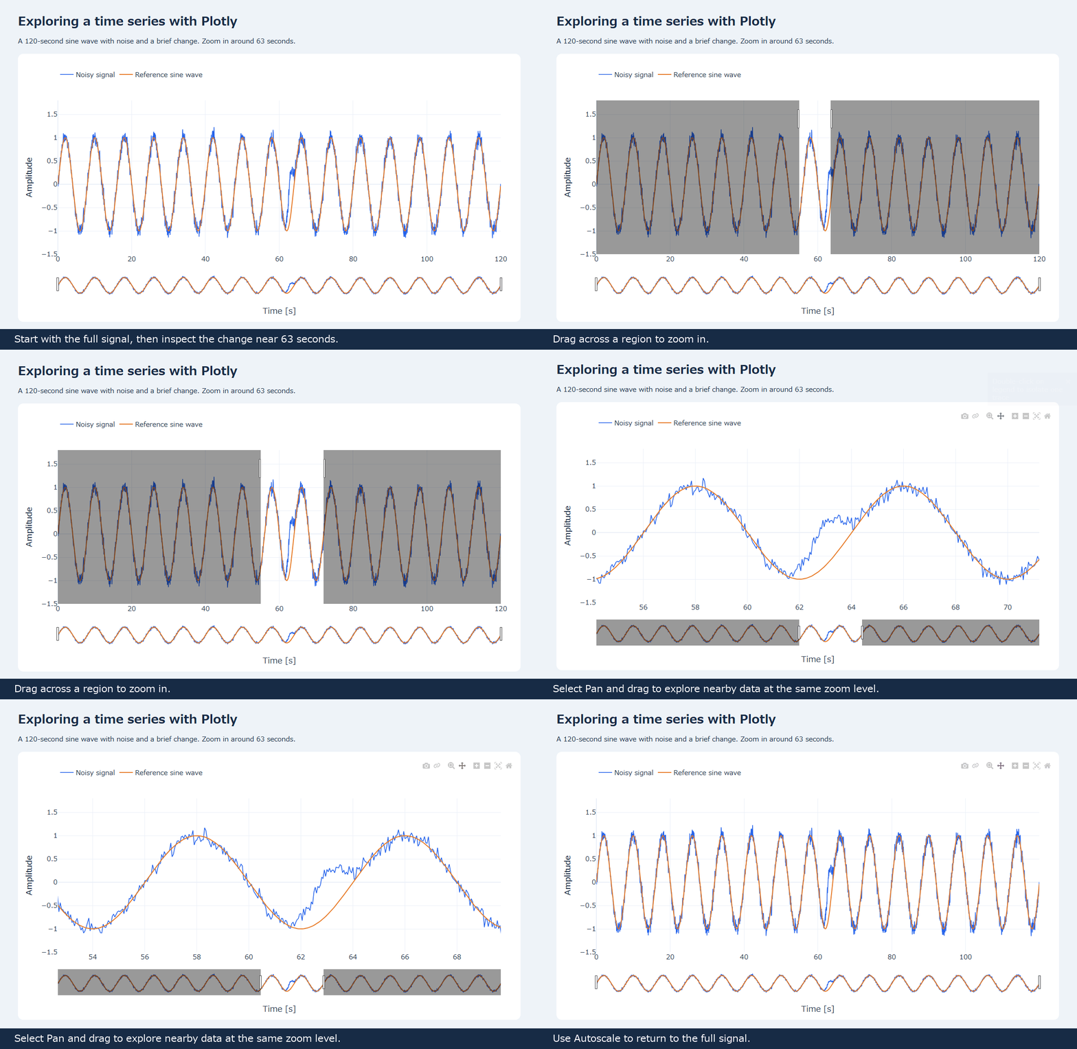
The change near 63 seconds is hard to pick out in the full view. Zooming in makes the difference from the reference sine wave easier to see. You can also hover to read values and click the legend to toggle a trace.
The GIF records those interactions. Open the HTML created by the code to explore whichever part interests you.
For measurement logs such as temperature or voltage, this could be a handy way to look at the overall trend, then investigate a particular moment in more detail.
In the follow-up, I made a CSV viewer that plots each data column separately with synchronized time axes. Zooming or panning one chart updates the others to the same interval. The article includes a GIF showing how you can compare measurement logs.
See you next time!


コメント