Hi, Higashi here.
In my last post, I used a CFD solver I wrote in Python to see how air moves through a U-shaped duct. I split the duct into cells 0.5 mm wide. What would I see if I halved that spacing? And if a coarser grid could tell me which side of the bend the fast air follows, how much time could I save?
I tried three grid spacings on the same duct, with the same airflow in each case. For the duct geometry and the Python code behind the calculation, see my earlier post, Can You Build a CFD Solver in Python? Simulating Airflow Through a U-Bend.
How much longer does a finer grid take?
The duct has a 6 mm × 6 mm square cross section. Air enters at 1 m/s and leaves at atmospheric pressure. I used the same RNG k–ε turbulence model as before, started each run from the same initial conditions, and let the flow settle.
| Grid spacing | Fluid cells | Solver runtime | Peak speed anywhere in the duct |
|---|---|---|---|
| 1 mm | 2,954 | 0.49 s | 1.63 m/s |
| 0.5 mm (original) | 19,872 | 7.81 s | 1.82 m/s |
| 0.25 mm | 158,976 | 196.44 s (3 min 16 s) | 1.92 m/s |
Going from 0.5 to 0.25 mm gave me exactly eight times as many cells. Halving the spacing doubles the count in each of three directions, so the total grows by 2 × 2 × 2. The 1 mm grid is the only one where some walls cut through cells. I counted each cell that contained air and took part in the calculation, even if air filled only part of it.
The finer run took about 25 times as long. There were more cells to update, and the solver also had to take smaller time steps. It took 2,200 steps for the flow to settle on the 0.5 mm grid and 5,000 on the 0.25 mm grid.
I timed one run per grid on the same PC, from setting up the pressure matrix until the solver reached its convergence criteria. For this comparison I used Numba to speed up the calculations between cells. I also used the fact that the duct has the same outline at every height to simplify the pressure solve. I reran the 0.5 mm case with these changes and checked that it reproduced the speed distribution from the earlier post. The timings exclude the first compilation, mesh generation, saving files and plotting.
Where does the fast air go after the bend?
These are top views of a horizontal slice halfway up the duct. Air comes in at the lower left, makes two right-angle turns at the far end and flows back to the outlet at the upper left. All three plots use the same color scale. Yellow marks the fastest air.
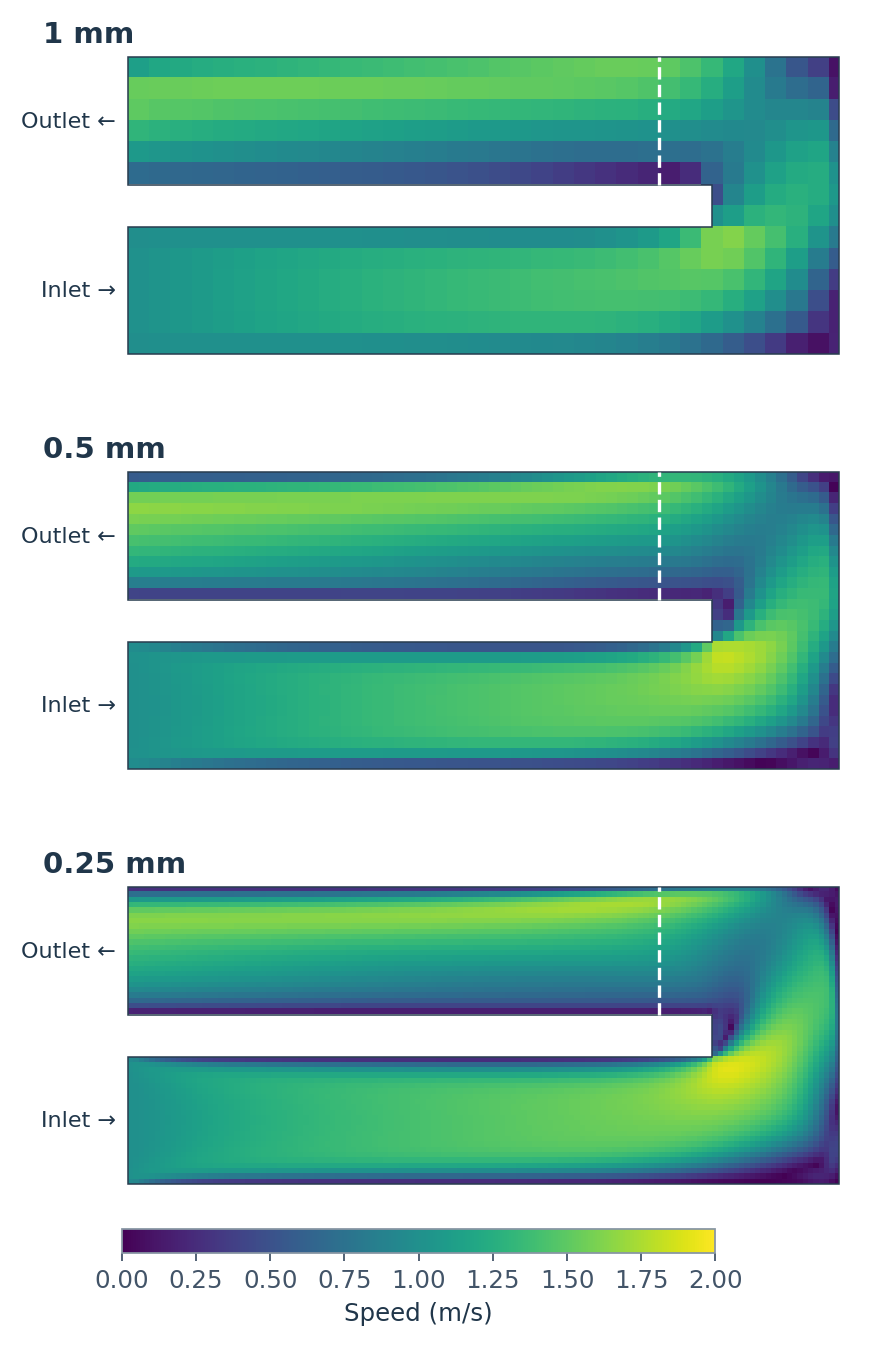
Look at the top leg of the 1 mm plot first. After the turn, the faster air runs along the outside of the bend, near the top edge of the plot. You can see the same pattern on both finer grids. If all I want to know is which side carries the faster air, the 1 mm grid already gives me an answer for this duct.
How much detail can we see near the outer wall?
Now take just the dashed line. It crosses the return leg 2.5 mm downstream of the inner corner. On the horizontal axis below, 0 mm is the inner wall and 6 mm is the outer wall. The air speed at each wall is fixed at zero.
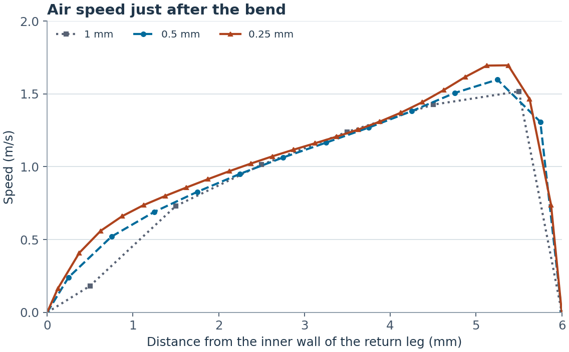
The three curves nearly overlap in the middle of the duct. Follow them toward the outer wall and the difference becomes easier to see. The highest speed along this line rises from 1.52 m/s on the 1 mm grid to 1.60 m/s at 0.5 mm and 1.70 m/s at 0.25 mm. On the coarsest grid, the last cell before the wall is also the fastest. On the finest grid, the peak sits about 0.6 mm from the outer wall, and there are several points to show how the air slows down from there.
How different are the runs across the whole duct? I averaged the finer grid’s velocity vectors over the volume of each corresponding coarse cell, then calculated the volume-weighted root-mean-square difference. It was 0.121 m/s between the 1 and 0.5 mm grids and 0.094 m/s between the 0.5 and 0.25 mm grids. As a percentage of the 1 m/s inlet speed, the difference fell from about 12.1% to 9.4%. These numbers measure agreement between grids. It would take a comparison with measured airflow to say how closely the finest grid matches the real duct.
Which grid would I use for this duct?
I’d use 1 mm for a first look at where the faster air goes. If I were changing the shape of the bend and comparing one design with the next, I’d use 0.5 mm. Each run took about eight seconds here.
If I needed to know how far the peak sits from the wall, I’d also run the 0.25 mm grid. The three color maps tell much the same story at a glance. A single line across the return leg shows what those extra minutes of computation actually buy.


コメント