Hi, Higashi here.
Where does air move fastest after it goes around a bend? Looking at the outside of a pipe, it’s hard to tell whether the fastest air stays near the middle or shifts to one side.
Computational fluid dynamics (CFD) gives us a way to investigate that. There are plenty of CFD packages, but the cost of a commercial license can be a hurdle when you just want to try an idea at home. That got me wondering: could I write the solver itself in Python?
The duct and the flow conditions
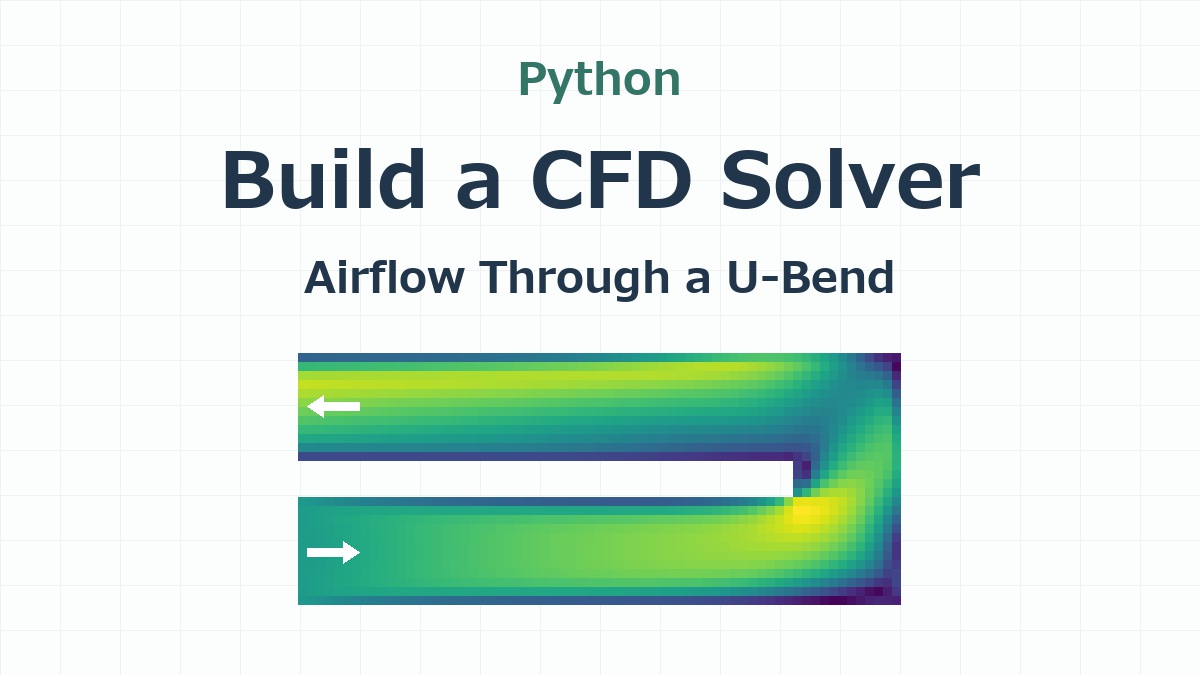
I used a duct with a square cross section, 6 mm wide and 6 mm high. Seen from above, it looks like a U lying on its side. Air enters the lower leg, travels to the right, makes two 90° turns, and returns along the upper leg.
| Item | Setting |
|---|---|
| Geometry | 33.5 × 14 mm in plan view, with a 2 mm wall separating the two legs |
| Mesh | 0.5 mm Cartesian grid, with 12 × 12 cells across the duct and 19,872 fluid cells in total |
| Inlet and outlet | Uniform inlet velocity of 1 m/s. Atmospheric pressure at the outlet (0 Pa gauge). |
| Walls | Solid, stationary walls with no slip. The air velocity at the wall is zero. |
| Numerical method | Three-dimensional incompressible flow, solved with the finite volume method |
| Turbulence model | RANS with the RNG k–ε model. I assumed a turbulence intensity of 3% at the inlet. |
The finite volume method divides the duct into small boxes called cells. For each cell, we keep track of how much air and momentum pass through its faces. The solver also handles cut cells. If a wall cuts through a cell, the calculation uses the volume occupied by air and the open area connecting it to each neighbor. For this particular duct, all the walls line up with faces of the 0.5 mm grid.
I wanted to try implementing a turbulence model in Python, too. The RNG k–ε model solves for the turbulent kinetic energy, k, and its dissipation rate, ε, alongside velocity and pressure. The Reynolds number based on the duct width and inlet speed is about 383, so I would expect laminar effects to dominate in this example.
Where does the fastest air go after the bend?
Here’s the calculated velocity field.
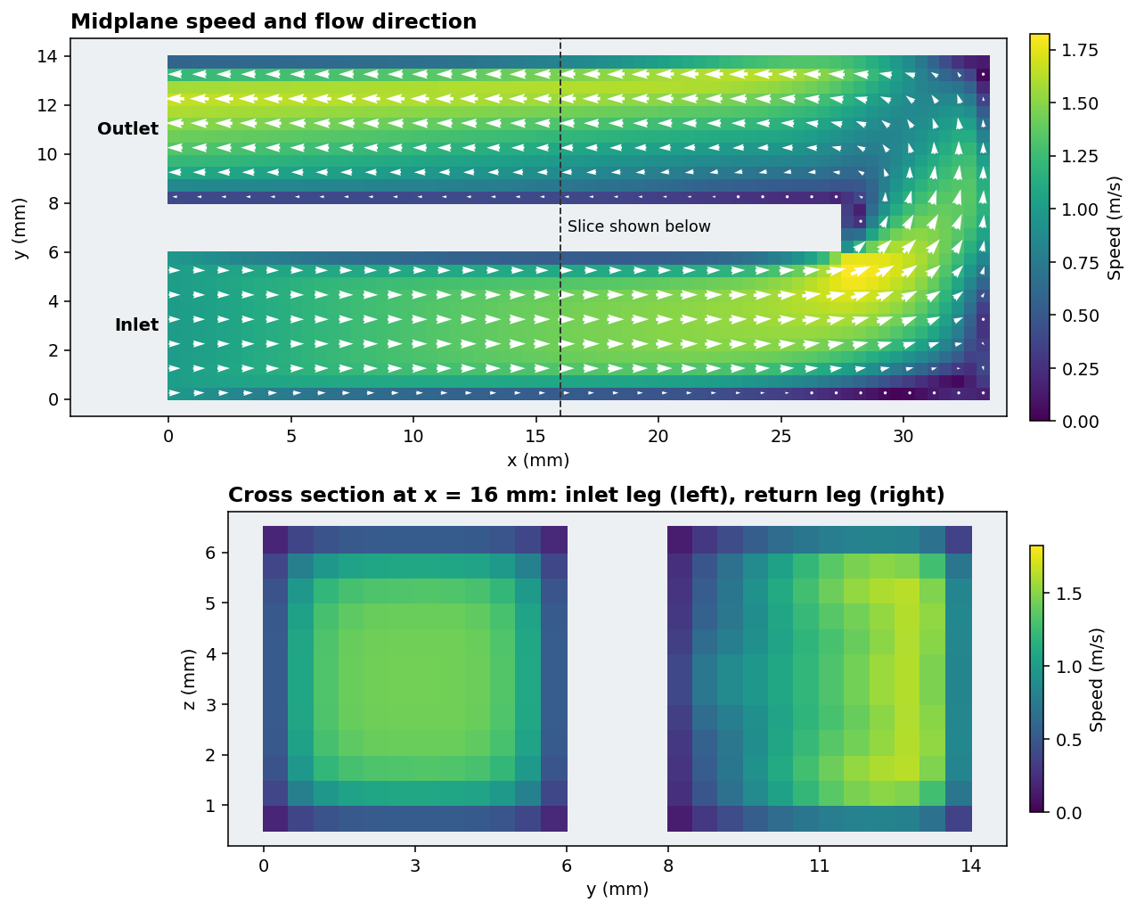
In the top plot, yellow means faster air, and the white arrows show the flow direction in the plane. Follow the arrows from the lower left: they run to the right, turn at the far end, and head back to the outlet at the upper left.
The two squares in the lower plot are the part I found interesting. The one on the left cuts through the inlet leg, before either turn. The one on the right cuts through the return leg, after both turns.
In the inlet leg, the air near the walls is slow, and the faster region sits roughly in the middle. In the return leg, the faster region has shifted to the right, toward the outside of the U. Both squares have the same area and carry the same flow rate, yet the fastest air is in a different place.
How does one cell exchange information with the next?
Let’s set aside most of those 19,872 cells for a moment and look at just two neighbors, A and B. They share a face measuring 0.5 mm by 0.5 mm. If air crosses that face perpendicularly at 1 m/s from A to B, the flow rate is 0.25 mL/s. The 0.25 mL leaving A each second is the very same 0.25 mL entering B.
That’s why the program calculates each face flow once and lets both cells use it. Here are the relevant parts of one time step. I’ve given a couple of intermediate results names to make the calculation easier to follow.
1. Use the velocity on the upstream side
The arrays f.i and f.j hold the indices of the two cells on either side of each internal face. Think of i as A and j as B. The volume flow rate through the face is q, with a positive sign for flow from A to B.
# Split the face flow into its A-to-B and B-to-A parts.
qplus = np.maximum(q, 0)
qminus = np.minimum(q, 0)

# Use the upstream velocity to find the momentum carried through the face.
advective_flux = qplus[:, None] * u[f.i] + qminus[:, None] * u[f.j]
If q is positive, qminus is zero, so only A’s velocity, u[f.i], contributes. If the flow reverses, only B’s velocity contributes. This choice of the upstream value is called upwinding.
Each velocity has three components, one for each axis. Writing qplus[:, None] lets NumPy multiply all three components by the flow rate for that face. The solver adds the viscous contribution, which depends on velocity differences between neighboring cells, to get the total momentum flux, momflux. The momentum equation is divided throughout by the constant air density.
2. Count the same flux as leaving A and entering B
We now have one momflux per face. To add up the contributions for each cell, the solver uses a matrix called internal. Its rows represent cells and its columns represent internal faces. In the column for the face shared by A and B, the entry is +1 in A’s row and −1 in B’s row.
# Sum outgoing minus incoming momentum flux for each cell.
net_mom = (
    internal @ momflux
    + bin_ @ in_mom
    + bout @ (qo_pos[:, None] * u[outlet.i])
    + bwall @ ((nu * wall_coef)[:, None] * u[wall.i])
)

# Divide by cell volume and advance the velocity by one time step, dt.
provisional = u - dt * net_mom / vol[:, None]
In Python, @ means matrix multiplication. The first term, internal @ momflux, sums the internal face contributions for every cell at once. The other three terms account for the inlet, outlet, and walls. For another example of using matrix multiplication in Python, see my earlier article on running a trained model with NumPy matrix multiplication.
The last line explains the signs. Momentum carried from A to B contributes with a plus sign to A’s net_mom and a minus sign to B’s. Since we subtract the net outgoing flux in the velocity update, A loses exactly the momentum that B receives.
3. Use pressure to balance the air entering and leaving each cell
The velocity we just calculated is called provisional for a reason. If we use it to calculate the flow rates, a cell may have more air entering than leaving. We’re treating air density as constant, so we solve for a pressure field that brings the inflow and outflow into balance in every cell.
# Interpolate cell velocities to faces. Normal velocity times area gives flow rate.
vf = interp(provisional)
base = area * vf[rows, f.a]
base_out = outlet.area * outlet.s * provisional[outlet.i, outlet.a]

# Find each cell's flow imbalance and solve for pressure using the outlet condition.
net = internal @ base + bin_ @ qi + bout @ base_out
pressure = solve_p(-net / dt + bout @ (out_stiff * pface))

# Correct the shared face flow using the pressure difference between A and B.
flux = base + dt * stiffness * (pressure[f.i] - pressure[f.j])
There are our two cells again in the last line. stiffness is the open face area divided by the distance between the cell centers. If A’s pressure is higher than B’s, pressure[f.i] - pressure[f.j] is positive, and the correction increases the flow in the A-to-B direction. Here, pressure is the solver’s pressure variable: static pressure divided by density, plus a turbulence term. The outlet value, pface, is set so that the static pressure there is atmospheric.
The corrected face flow, flux, becomes q in step 1 the next time around. That closes the loop: the upstream cell supplies the velocity for momentum transport, and the pressure difference between the neighbors adjusts how much air crosses their shared face.
How long did the calculation take?
For this case, the solver took 2,200 time steps and about 72 seconds to reach the stopping criteria. By then, changes in velocity, pressure, and the turbulence variables were small, and the flow rates balanced. The timing covers the solver itself.
We can check the result from the inlet dimensions alone. At 1 m/s, a 6 mm square opening admits 36 mL of air per second. The calculated outlet flow was also 36 mL/s, while the highest speed anywhere in the duct was 1.82 m/s.
So yes, I could build a Python CFD solver for a duct this size, starting with the calculation across a single cell face. My favorite part was taking that last slice through both legs. The inlet and outlet flow rates agree, but only the cross section shows how far to one side the faster air has moved.
See you next time!

コメント