
Hi, Higashi here.
Python is often the first choice for building an AI model. But installing new software is not always an option, and setting up an environment can be enough to put you off getting started.
Could we build an AI model using just the Excel we already have?
I tried building a small neural network in Excel VBA, loading data, training it, and making predictions on records it had not used for training. The model’s training and prediction calculations use no Python or additional add-ins.
Training and making predictions in Excel
The model takes 10 numerical inputs and returns one predicted number.
One way to picture this is predicting a measurement from the conditions under which it was taken. For this experiment, I used a public dataset so that I could check how the implementation behaved.
First, we use pairs of inputs and known answers to adjust the numbers inside the model so that its predictions get closer to those answers. This is training. After training, we keep those numbers fixed and use them to calculate an output from an input. This is prediction, also called inference.
VBA is often associated with copying cells and automating reports. But it also supports arrays, loops, and arithmetic, which are enough to implement these calculations.
The Diabetes dataset and a small MLP
I used the Diabetes dataset, which appears in machine learning examples. It contains 442 records with 10 input features: age, sex, BMI, average blood pressure, and six measurements related to blood tests. The target is a numerical measure of disease progression one year later. You can find the dataset description in the official scikit-learn documentation.
This is a regression problem: predicting a number rather than deciding whether someone has diabetes. The output is the dataset’s progression measure, not blood glucose in mg/dL.
For a closer look at matrix-based prediction, see my earlier article on running a trained MLP with NumPy matrix multiplication.
The model is an MLP, or multilayer perceptron, with layers connected in sequence. I used this small structure:
10 inputs → 8 hidden units → 1 output
The inputs are multiplied by weights and added together. The hidden layer applies a function called tanh, and the output layer produces the prediction. During training, backpropagation calculates how the weights should change, and an optimizer called Adam updates them. There are 97 adjustable parameters in total, including weights and biases.
| Item | Setting |
|---|---|
| Data split | 265 training / 88 validation / 89 test records |
| Hidden / output activation | tanh / linear |
| Weight updates | Adam using gradients from the full training set |
| Learning rate / L2 coefficient | 0.01 / 0.001 |
| Random seed | 42 |
Inputs with very different scales can make training harder, so both the inputs and the target are standardized before calculation. The means and standard deviations are calculated using only the 265 training records. Predictions are then converted back to the target’s original scale. This preprocessing also runs in VBA.
The training set is used to adjust the weights, the validation set helps decide when to stop and which model to keep, and the test set is used for the final evaluation. I wanted to check more than whether the model could fit the same records it had learned from.
How does the error change during training?
Here is the training history from the VBA program running in Excel. The horizontal axis shows epochs, and the vertical axis shows the prediction error measured as RMSE. In this implementation, one epoch means calculating gradients from the full training set and updating the weights once.
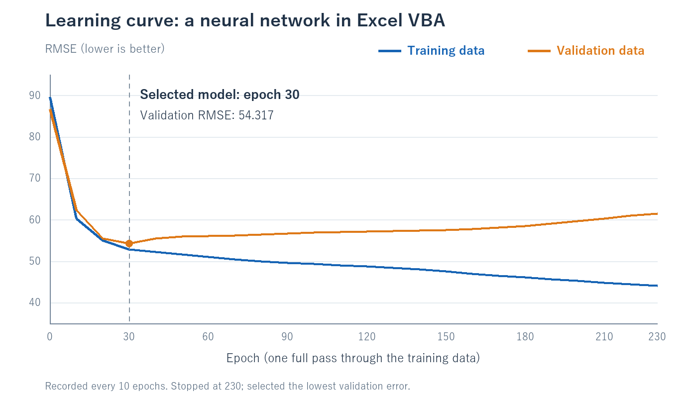
At first, both errors fall sharply. After about 30 epochs, however, the training error keeps decreasing while the validation error gradually increases.
This is a sign of overfitting: the model is fitting the training data more closely while making worse predictions on records it did not train on. More training is not always better.
I stopped training once the validation error had not improved for 200 epochs. The loop ran for 230 epochs, but the final model uses the weights from epoch 30, when validation error was lowest.
The vertical axis here is RMSE in the target’s original units. It is distinct from the training objective, which combines squared error on standardized targets with L2 regularization.
Predicting 89 records held out from training
I used the selected model to predict the 89 test records and compared the predictions with their actual values.
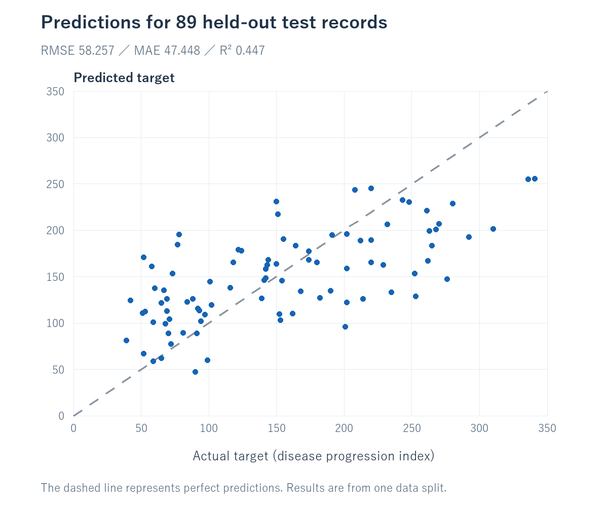
| Metric | Measured in Excel |
|---|---|
| Test RMSE | 58.257 |
| Test MAE | 47.448 |
| Test R² | 0.447 |
| Test RMSE when always predicting the training-set mean | 78.521 |
RMSE and MAE measure how far predictions are from the actual values; lower is better. An MAE of 47.448 means that the absolute prediction error averaged about 47.4 on this test set. R² is better when closer to 1, but an R² of 0.447 does not mean “44.7% accuracy.”
I also compared the model with a simple baseline that always predicts the mean target value from the training set. Its test RMSE was 78.521, compared with 58.257 for the MLP: a reduction of about 25.8% in RMSE. The model is using information from the inputs to do better than returning the same answer every time.
These results come from one data split. I have not compared the model with ordinary multiple linear regression on the same split. A more thorough assessment would compare models under the same conditions and repeat the evaluation with different splits.
Using the trained model for prediction
After training, the weights and biases can be extracted for use in matrix calculations. Combining them with the same standardization and activation functions used during training lets us predict outputs for new inputs. There is no need to train the model again for every prediction.
The VBA code that trains the neural network
Here is the training section extracted from the program I ran. Rather than focusing on loading data or creating charts, look at how it adjusts the weights.
This excerpt explains the calculation process. Variable declarations, data standardization, weight initialization, and helper functions are omitted, so it cannot run by itself if you simply paste it into VBA. The result-display code is also omitted.
These are the main variables used in the code:
| Variable | Meaning |
|---|---|
x(i, j) / y(i) |
Standardized inputs / target values |
w(k) |
The 97 weights and biases being adjusted |
grad(k) |
Gradients indicating how the parameters affect error |
a(k) |
Hidden-layer outputs: eight in this model |
moment(k) / variance(k) |
Moving averages of gradients and squared gradients used by Adam |
best(k) / bestLoss |
Weights with the lowest validation error / that error |
Before the loop, the 10 inputs and the target have been standardized, and the weights have been initialized. Adam’s moving averages start at 0, while b1Power and b2Power start at 1. The initial weights and validation error are stored in best and bestLoss, and bestEpoch starts at 0.
' Calculate full-batch gradients and update the weights
For epoch = 1 To MAX_EPOCHS
    For k = 1 To P: grad(k) = 0#: Next k
    ' Backpropagate prediction errors through the output and hidden layers
    For i = 1 To nt
        e = Forward(x, i, w, a) - y(i)
        grad(P) = grad(P) + e
        For k = 1 To H
            grad(H * (D + 1) + k) = grad(H * (D + 1) + k) + e * a(k)
            dh = e * w(H * (D + 1) + k) * (1# - a(k) * a(k))
            offset = (k - 1) * (D + 1)
            grad(offset + D + 1) = grad(offset + D + 1) + dh
            For j = 1 To D: grad(offset + j) = grad(offset + j) + dh * x(i, j): Next j
        Next k
    Next i
    ' Update with Adam; apply L2 regularization to weights, not biases
    b1Power = b1Power * 0.9: b2Power = b2Power * 0.999
    For k = 1 To P
        grad(k) = grad(k) / nt
        If Not BiasParameter(k) Then grad(k) = grad(k) + L2 * w(k)
        moment(k) = 0.9 * moment(k) + 0.1 * grad(k)
        variance(k) = 0.999 * variance(k) + 0.001 * grad(k) * grad(k)
        w(k) = w(k) - LEARNING_RATE * (moment(k) / (1# - b1Power)) / _
               (Sqr(variance(k) / (1# - b2Power)) + 0.00000001)
    Next k
    ' Validate every 10 epochs and retain the best weights
    If epoch Mod CHECK_EVERY = 0 Then
        trainLoss = MSE(x, y, 1, nt, w)
        valLoss = MSE(x, y, nt + 1, nt + nv, w)
        If valLoss < bestLoss - 0.0000001 Then
            bestLoss = valLoss: bestEpoch = epoch
            For k = 1 To P: best(k) = w(k): Next k
        End If
        ' Stop after 200 epochs without a validation improvement
        If epoch - bestEpoch >= PATIENCE Then Exit For
    End If
Next epoch

' Restore the weights with the lowest validation error
For k = 1 To P: w(k) = best(k): Next k
Use prediction errors to calculate gradients
e = Forward(x, i, w, a) - y(i) calculates the difference between the current prediction and its target. Forward is a helper function that calculates the hidden layer and then the output from the inputs.
The following additions to grad perform backpropagation. They propagate the output error back through the hidden layer to calculate how changing each weight affects the error. The term 1# - a(k) * a(k) is the derivative of the hidden layer’s tanh activation.
Combine gradients from 265 records and update with Adam
For i = 1 To nt loops over all 265 training records, and grad(k) / nt calculates the average gradient. Adam then updates w(k), using previous gradients to adjust the size of the update.
BiasParameter is a helper function that identifies bias parameters. L2 regularization, which discourages excessively large weights, is applied to weights but not biases. The learning rate is 0.01, and the L2 coefficient is 0.001.
This implementation combines all 265 records into one weight update rather than updating after each record. Repeating that process produced 230 updates in this run.
Use validation data to decide when to stop
MSE is a helper function that calculates the mean squared error for a specified range of records. Every 10 epochs, the program checks the error on the 88 validation records and saves the weights in best if the error improves. Validation records are not used to calculate gradients for updating weights.
If the validation error does not improve for 200 epochs, the loop stops. Finally, w(k) = best(k) restores the best weights. This is why the program ran for 230 epochs but selected the model from epoch 30. The evaluation on the 89 test records happens separately, after model selection is complete.
The squared errors in the code use standardized targets. For the graph, I took the square root and converted back to the original target scale to display RMSE.
So the cycle of making predictions, measuring errors, and adjusting weights can be written in VBA. I checked the implementation in desktop Excel for Windows. Excel for the web cannot run VBA macros.
Execution time and what makes Excel interesting here
The training loop took 0.500 seconds, measured with VBA’s Timer function. This is one measurement covering 230 epochs of weight updates, intermediate validation, and history logging. It excludes CSV loading, preprocessing such as standardization, and the creation of the final results table and charts. The experiment is small: 442 records and eight hidden units.
Python libraries will often be easier to work with when handling large datasets or comparing many different model types. But at this scale, Excel VBA was enough to run both training and prediction.
It is interesting to be able to inspect the inputs, training history, predictions, and model weights in the same workbook. That could also make a useful learning exercise: change a setting and see how the predictions respond.
If you are interested in AI but unsure where to begin, why not start by exploring how to build and use an AI model in Excel?
See you next time!


コメント